Medical Costs Analysis using a Linear Regression model

This will be my first announcement. For the beginning, let’s see how to use Python and to build a simple Linear Regression model to predict some data. In this example, it will be presented how to simply analyze a raw data and to use regression model for the purpose of analyzing the Medical Costs Data. The data is obtained from link.

The task will be to perform all the necessary steps which are required for successful implementation of a machine learning model: to load the data, to learn from the data, to analyze information and graphically represent numerical categories, to convert object categories to label (dummy) variables, to import and fit Linear Regression models, to predict values using the fitted model, and finally, to measure accuracy of the model.

• First, let’s import required libraries for further work.

    import numpy as np
    import pandas as pd
    import seaborn as sns
    import matplotlib.pyplot as plt

• Next step is to load the dataset.

    df = pd.read_csv("../input/insurance.csv")

• The most important thing at the beginning is to understand the data. There is no point in building machine learning models if we do not understand what are we looking for in our data and what are our expectations. Let’s see some basic information about data set.

• Which categories are included in our data set?

    df.columns

• We will print the first five rows of our DataFrame to see how our data look in the table.

    df.head()

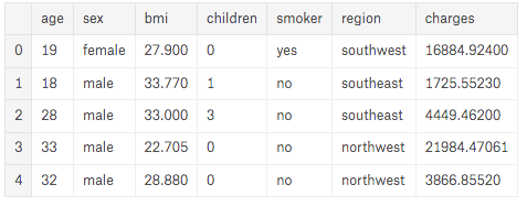
As we can see, 7 different categories are presented through the data.

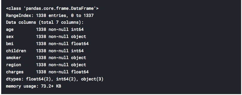
• Next, a number of entries for each category and types of data are presented. We have at our disposal 4 numerical and 3 object categories.

    df.info()

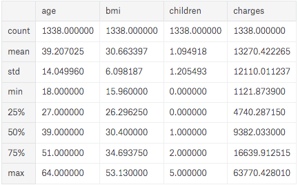
• The function “describe” will present characteristics of all numerical categories.

    df.describe()

• Next part is to graphically represent our numerical data. We will plot pairplot graph from the seaborn library.

    sns.pairplot(df)

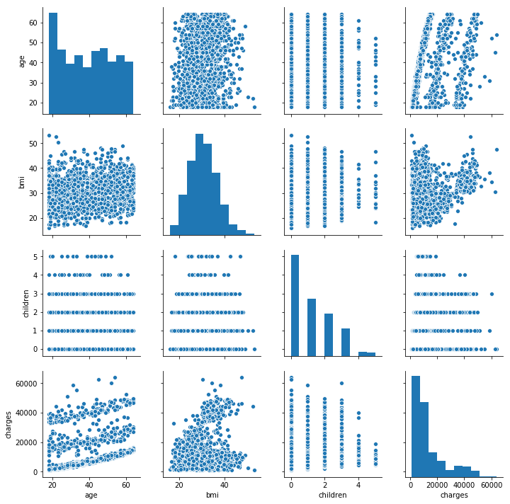
Pairplot is the easiest way to see all mutual correlations between different categories and distributions of data for each category separately, for all numerical categories.

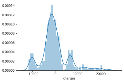
• Let’s now suppose that the variable of interest is “charges”. We want to predict what would be medical costs for specific individual, based on other given information. Let’s see distribution of data for “charges”.

    sns.distplot(df["charges"])

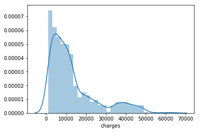
From the figure above we can conclude that the variable “charges” do not possess normal distribution of data, but it has a mixture distribution. That could be a problem for getting optimal performances of our model, and we will see in the next announcement how we can easily deal with this problem.

• Next figure is a heatmap. It represents mutual correlation of numerical categories from our dataset.

    sns.heatmap(df.corr(),annot=True)

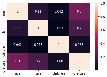
And we have found 1st interesting fact: Children category (Number of children covered by health insurance) has the lowest correlation with “charges”. Personally, I thought it would be vice versa.

• As it is said, three object categories are included. What could be done to analyze that kind of data? For example, “region” category could be summed up as:

    df['region'].value_counts()

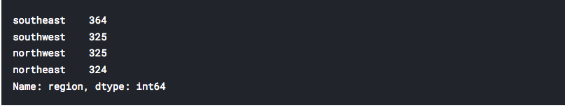
We could determine within each categorical variable what is the number of impressions for each specific category, as we did with the “region”. But how to present all these categories in the way to be suitable for processing together with our numerical variables? One hot encoding is the answer.

One hot encoding is the procedure of transforming categorical variables as binary vectors. How does it works? Let’s back to the “region” category. Each individual must be part of one of the four regions:

$$[southeast, southwest, northwest, northeast]$$

One hot encoding will transform affiliation to a specific region to the vector of four elements, for example:

$[0,0,1,0]$ - Third element is 1, so this individual is from the northwest. After that, next person region information is transformed to:

$[1,0,0,0]$ - of course, this is someone from the southeast. Simple as a cake!

What next? To transform categorical variables sex, smoker and region by using One hot encoding, and add obtained categories to our dataframe.

    sex_dummy = pd.get_dummies(df['sex'])
    smoker_dummy = pd.get_dummies(df['smoker'])
    region_dummy = pd.get_dummies(df['region'])

    df = pd.concat([df,sex_dummy,smoker_dummy,
                    region_dummy], axis=1)

    df.rename(columns={'no': 'non-smoker',
              'yes': 'nicotian'}, inplace=True)

• We have successfully transformed our categorical variables, so we can remove these original categories from our DataFrame.

    df = df.drop(['sex','smoker','region'], axis=1)

In the table below we can easily recognize our new (One hot encoding) columns.

    df.head(10)

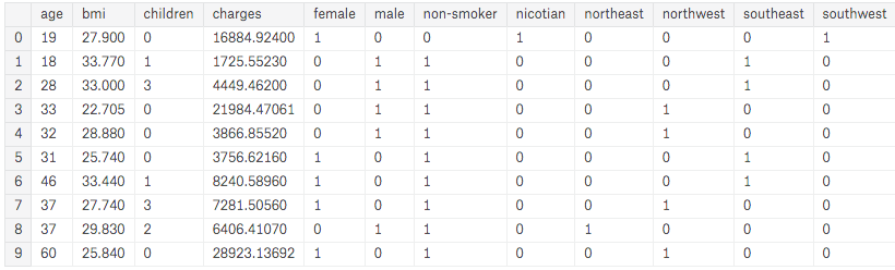
Now we can use all 7 initial categories for prediction purposes.

• We have prepared our data for processing and fitting a new model. Next part is to use function train_test_split to divide all information in the two subsets: training and testing.

    from sklearn.model_selection import train_test_split

• Eleven data-frame categories will be used as inputs of the model. We want to fit our model according to the “charges” category, so output variable Y will be “charges” of course.

    X = df[['age', 'bmi', 'children',
    'female','male','non smoker',
    'nicotian','northeast','northwest',
    'southeast','southwest',]]

    y = df['charges']

• Usage of train_test_split function

    X_train, X_test, y_train, y_test =
    train_test_split(X, y, test_size=0.4)

• Finally, we can proceed with the procedure of importing and fitting the Linear Regression model.

    from sklearn.linear_model import LinearRegression
    lm = LinearRegression()
    lm.fit(X_train,y_train)

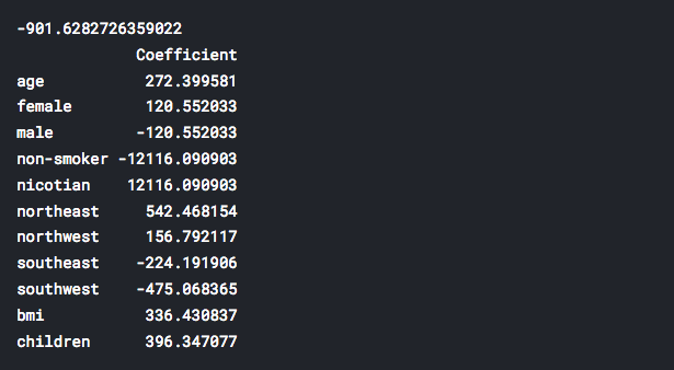
• The model is fitted. We will create a new data-frame to present estimated coefficients obtained by our model. Each coefficient represents one specific category. First number (above the coefficients) is the intercept term of our fitted linear regression model.

    print(lm.intercept_)

    coeff_df = pd.DataFrame(lm.coef_,X.columns,
    columns=['Coefficient'])

    print(coeff_df)

• Interesting fact 2: Quit smoking! We can observe that the nicotian category (from the table above) has the highest influence on medical costs calculations. On the contrary, non-smoker category possess the largest negative influence on medical costs. Do you need any more concrete reason what are the benefits of being non-smoker? Smoker/non-smoker categories possess stronger influences than all other analyzed parameters TOGETHER.

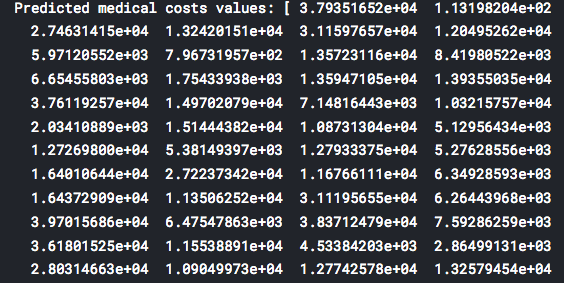
• Final part of this short case study is to test the trained model for predicting a new “charges” values (by using prepared X_test data which is obtained by train_test_split function)

    predictions = lm.predict(X_test)
    print("Predicted medical costs values:", predictions)

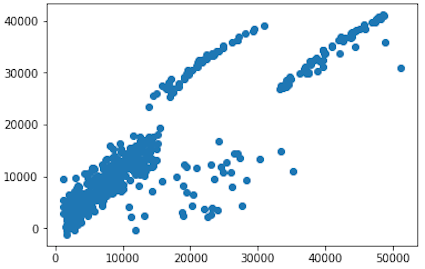
• We will present graphical comparison of expected values of our analysis (y_test) and predicted values (predictions) of our trained model.

    plt.scatter(y_test, predictions)

• Also, let’s see an error distribution graph of our predictions.

    sns.distplot((y_test-predictions), bins=50)

• Finally, let’s calculate and print mean absolute error (MAE) and mean squared error (MSE) for our predictions. These measures will represent quality parameters of our model (achieved prediction accuracy).

    from sklearn import metrics
    print(metrics.mean_absolute_error(y_test, predictions))
    print(metrics.mean_squared_error(y_test, predictions))

That’s it for the beginning. As we can see from calculated errors, our model is far from perfect. There are definitely better machine learning models which could be used for achieving better prediction performances, but the point in this text was to present how to predict using Linear Regression.

So, is there any way to improve obtained performances and to keep the proposed model? Yes, there is a way. We will see in the next announcement how one simple transformation of “charges” category could dramatically increase performances of our model.